Applications of Control Theory in Network Epidemiology: Modeling, Optimization, and Parameter Estimation

Understanding the dynamics of disease outbreaks is pivotal for the development of methods for their mitigation and control, both in the presence and absence of treatments and vaccines. With the COVID-19 Outbreak still ongoing, the development of scientific tools and mathematical models for epidemics and spreading processes has seen a global effort in multiple fields.

The field of Control Theory is known for its wide applications in all areas of science that encapsulate dynamical systems, and so it is no surprise that its notions are of utility in the analysis and control of spreading processes over populations.

The study of spreading processes dates back to the 1700s, when Bernoulli developed one of the first known epidemic models in an attempt to understand the growth of the smallpox virus. In 1927, the well-known Susceptible-Infected-Susceptible (SIS) and Susceptible-Infected-Recovered (SIR) Models were introduced by Kermack and McKendrick. They have constituted the most intuitive sets of differential equations used to illustrate the dynamics of a spreading process. These equations express the rate of increase or decrease of each of three states in a population (Susceptible, Infected, Recovered/Removed) in terms of the current states. The spreading process is tied to two values, known as spreading parameters: the infection rate and the recovery rate. Mathematically, these rates can be interpreted as rates for Poisson Processes, one for infections and one for recoveries. The ratio of these parameters gives what is known as the Basic Reproductive Number, a standard metric in analyzing disease stability.

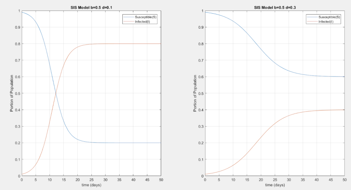
Kermack-McKendrick SIS Model Simulations for homogeneous population starting with 99% Susceptible and 1% Infected, where b is the infection rate and d the recovery rate. Clearly, the disease dynamics depend on the ratio between b and d as illustrated in the different steady-state values in the two simulations.

However, the Kermack-McKendrick Models fail in practice as they assume that the graph describing the population network is completely connected, meaning that every individual in the population is connected to every other individual. This assumption is too strong, and therefore a population network is added to the model. This population network is based on Graph Theory notions, and so it is expressed in terms of an Adjacency Matrix defining the existence and weight of edges between nodes. The nodes in the graph can be used to represent individuals, or maybe even metapopulations (clusters of individuals that follow the Kermack-McKendrick Model). 

The standard Networked SIS model is obtained by doing a mean-field approximation on a much more complex 2n-Markov Chain Model, where n is the number of nodes, and the two states 0 and 1 represent a healthy and infected node respectively. The model is coupled with recovery and infection rates as in the Kermack-McKendrick Model, as well as an adjacency matrix describing the population network, which ultimately define the dynamics of the spreading process. Thus, the standard model used throughout analysis, optimization, and parameter estimation is known as the N-Intertwined Mean-Field Approximation (NIMFA) Model. The NIMFA Model allows for heterogeneity in the system parameters, and so it is now also possible to define different spreading parameters for each node. Hence, it is possible to differentiate between nodes in the network in terms of their importance in the dynamics of the disease spread by observing their interconnections with other nodes and their respective spreading parameters.[2]

The SIS NIMFA Model is expressed using n nonlinear differential equations describing the probability that each node is infected, or in the metapopulation case where it is assumed that each node represents a small population, the portion of individuals that are infected. Thus, the variables under study are all between 0 and 1. The model can be discretized and simulated through numerical methods such as Euler’s Method or higher Runge-Kutta schemes.

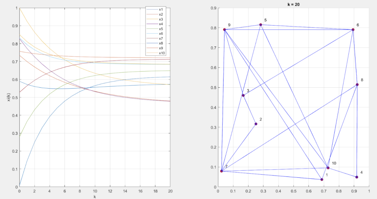
Simulation of a discretized SIS NIMFA Model with for a 10-node network over a 20-day period. The infection and recovery rate are chosen as 0.05 and 0.075, respectively, for all nodes. The graph adjacency matrix and initial conditions are randomly generated. We show the graph and a snapshot of the node states on the 20th day, where the node color represents the probability of infection (blue represents 0 probability, red represents 1 probability).

Due to the nonlinearity of the system, it is inefficient to obtain explicit expressions of the dynamics of the spreading process. It is of interest, instead, to confirm the existence of a Disease-Free Equilibrium (DFE) and the stability of that equilibrium state. This is done by resorting to results from Lyapunov Stability Theory, which is widely used in Nonlinear Control Analysis [3]. Namely, a necessary and sufficient condition for stability of the DFE is obtained. It states that the largest real part of the eigenvalues of the matrix BA – D must be negative. The matrices B and D are, respectively, the diagonal matrices of infection and recovery rates for each node, whereas A is the adjacency matrix of the graph representing the network structure. This stability condition can be extended to cases of time-varying networks in which the spreading parameters may vary over time to account for mutations in the disease (increase in infection rate, decrease in recovery rate)  or the discovery of a new treatment/vaccine (increase in recovery rate). It is also possible to introduce a time-varying adjacency matrix to account for periodic quarantine and social distancing measures. [4]

The conditions for stability of the DFE in the system are used as benchmarks in developing measures to ensure a given system’s eradication of the disease by changing control variables. The control variables are the adjacency matrix, and if possible, the recovery rate. Namely, controlling the adjacency matrix corresponds to implementing social distancing and quarantine measures, which ensure that contact between the nodes is reduced. On the other hand, increasing the recovery rate corresponds to finding a treatment or a vaccine for increased immunity. One way to do that is by implementing quarantine, or in a way decreasing the entries of the adjacency matrix, implying physically that contact between nodes is reduced. Another method is increasing the recovery rate, physically implying a treatment, vaccine, or increase of immunity. Since any treatment or vaccine is of a limited availability, we face an optimization problem aimed at picking the best nodes to treat, e.g. the nodes with the most connectivity. This type of optimization problems is known as a resource allocation problem.[5] In many cases, it can be impossible to reach the eradication of the disease, and so the choice of the control variables aims at minimizing the steady-state values given the boundaries of the control variables.

In addition to analysis and optimization, a third aspect of control theory and system identification that can be relevant to epidemiology is the wide subfield of Parameter Estimation. Given data on the recoveries and infections in a certain population, there exist methods for estimating the spreading parameters and even the network’s adjacency matrix through least square methods and maximum likelihood estimations. [6]

At the AUB Control and Optimization Lab, I am working under the supervision of Dr. Abou Jaoude to adapt and apply the techniques from control theory summarized in this article to model and increase the understanding of the COVID-19 outbreak in the context of Lebanon.

Filters: Control Theory; Network Epidemiology; Epidemiology; COVID-19

Contributors

[1]: Control Theory and Engineering Student – AUB Control and Optimization Lab, Department of Mechanical Engineering

References

[2]: Mieghem, P. V., Omic, J., & Kooij, R. (2009). Virus Spread in Networks. IEEE/ACM Transactions on Networking, 17(1), 1-14. doi: 10.1109/tnet.2008.925623

[3]: Pare, P. E., Beck, C. L., & Nedic, A. (2018). Epidemic Processes Over Time-Varying Networks. IEEE Transactions on Control of Network Systems, 5(3), 1322-1334. doi: 10.1109/tcns.2017.2706138

[4]: Preciado, V. M., Zargham, M., Enyioha, C., Jadbabaie, A., & Pappas, G. J. (2014). Optimal Resource Allocation for Network Protection Against Spreading Processes. IEEE Transactions on Control of Network Systems, 1(1), 99-108. doi: 10.1109/tcns.2014.2310911

[5]: Slotine, J. E., & Li, W. (2005). Applied Nonlinear Control. Taipei: Prentice Education Taiwan.

[6]: Vrabac, D., Pare, P. E., Sandberg, H., & Johansson, K. H. (2020). Overcoming Challenges for Estimating Virus Spread Dynamics from Data. 2020 54th Annual Conference on Information Sciences and Systems (CISS). doi: 10.1109/ciss48834.2020.1570627764